Table of Contents

• Sample Averaging And Epsilon Greedy Exploration
• Convergence to Correct Values
• Average Performance Over Multiple Problems

Consider a gambler sitting down at a row of slot machines. The gambler must make a choice of which slot machine to play. Every slot machine has an arm which can be pulled. For each pull, the machine returns some reward.

The returned reward is not constant on each machine. If it were constant, the gambler could simply pull every arm once, see which arm returned the highest reward, and then pull that arm continuously. Instead, each arm returns a reward sampled from a random distribution. In theory, the distribution can be any probability distrubtion. For simplicity, we will assume the reward returned by the machine is a normal distribution with standard deviation 1 centered at some random value and that it does not change over time. For example, an individual arm may have a random distribution centered at 0.5, which returns a random value from a normal distribution centered at 0.5 with standard deviation 1 when pulled.

The above problem is known as the Multi Armed Bandit problem. It's known by that name because slot machines are sometimes known as one-armed bandits. Here is an implementation of such a bandit in python with numpy.

"""bandits.py"""
import numpy as np


class Bandit:
    def __init__(self, num_arms: int):
        self.num_arms = num_arms

        # The action value of each arm is chosen from a normal distribution with
        # standard deviation 1 centered at 0.
        self.values = np.random.normal(size=num_arms)

        self.optimal_arm = np.argmax(self.values)

    def pull(self, arm: int):
        """
        Pull the arm at index 'arm'.

        The return value for each arm is a normal distribution with standard deviation 1
        centered at whatever the action value is for that arm.
        """
        return np.random.normal(self.values[arm])

    def is_optimal_arm(self, arm: int):
        """
        Returns true if the provided arm index is the optimal arm. Otherwise returns false.
        """
        return arm == self.optimal_arm

Sample Averaging And Epsilon Greedy Exploration

The gambler's goal is to maximize the reward they will receive by playing the slots. Initially the gambler has no idea which arm is optimal. However, the agent can use the returned value from each arm to form estimates of each arm's expected value. Once the agent has an estimate of the values for each arm, it must then make a choice about which arm to pull. The estimated value for each arm $a$ is represented by $Q(a)$.

The method chosen to make these estimates is known as an action-value method. I'm going to use the sample averaging action value method to estimate the action values. The sample averaging method is defined as the running average value returned for each arm. For a particular arm $a$ we have

The sample averaging method has a very nice property. The existing estimate for a particular arm can be updated incrementally. That is, it can be updated using only the previous estimate and the current reward. The property guarantees that the update to each estimate can occur in constant time and with constant memory. This can be seen in the following formula for an arm which has been pulled $n$ times.

Sample averaging provides a way of estimating the action values. Once we have an estimate, we then need a method to make a choice about which arm to pull. The obvious strategy is to choose the arm we currently think is optimal. However, it may be the case that our current best guess is not actually the optimal arm and that with repeated choices we may find another arm is better. If we always choose the arm we think is optimal, we eliminate any possibility of finding another more optimal arm. Additionally, continuing to explore once we are very confident in the estimated values will lead to sub-optimal performance. This problem is known as the exploitation vs exploration dilemma.

One method of choosing an arm to pull is known as the $\epsilon$-greedy method. It balances the exploitation vs exploration problem by choosing the arm we currently think is best most of the time, and a random arm some other percentage of time. The percentage of time spent exploring is denoted $\epsilon$. I.e.

A higher value of $\epsilon$ means the agent will explore more often and more quickly get accurate values estimates for each arm. At the same time, the more time spent exploring is the more time spent not exploiting the best arm. In general, a higher $\epsilon$ will converge more quickly but have a lower percentage of time choosing the optimal arm and vice versa for a lower $\epsilon$.

Here is an implementation of such an agent using $\epsilon$-greedy exploration with sample averaging updates.

"""agents.py"""
import numpy as np


class Agent:
    def __init__(self, bandit: Bandit, epsilon: float, time_steps: int):
        self.bandit = bandit                                # Instance of Bandit
        self.estimated_values = np.zeros(bandit.num_arms)   # ndarry containing the current estimates Q(a)
        self.chosen_count = np.zeros(bandit.num_arms)       # ndarry containing the number of times each arm was pulled
        self.epsilon = epsilon                              # Epsilon value in epsilon-greedy. How often to explore

        self.total_steps = 0
        # 2d array containing the estimated values at each time step
        self.tracked_estimated_values = np.zeros((time_steps, self.bandit.num_arms))

    def update_estimates(self, reward: float, arm: int):
        """
        Update estimates using the incremental update method and sample averaging.

        $$
        Q_{n+1} = Q_{n} + \frac{1}{n}\left[ R_{n} - Q_{n} \right]
        $$
        """
        self.chosen_count[arm] += 1
        self.estimated_values[arm] = self.estimated_values[arm] + (1/self.chosen_count[arm]) * (reward - self.estimated_values[arm])

    def step(self):
        """
        Pull an arm and update the estimates.
        """
        # Epsilon greedy exploration
        if np.random.random_sample() < self.epsilon:
            arm = np.random.randint(self.bandit.num_arms)
        else:
            arm = np.argmax(self.estimated_values)

        # Pull the arm and update estimates based on the reward
        reward = self.bandit.pull(arm)
        self.update_estimates(reward, arm)

        # Other tracking for graphs and stuff
        self.tracked_estimated_values[self.total_steps] = self.estimated_values
        self.total_steps += 1

        return reward, self.bandit.is_optimal_arm(arm)

Convergence to Correct Values

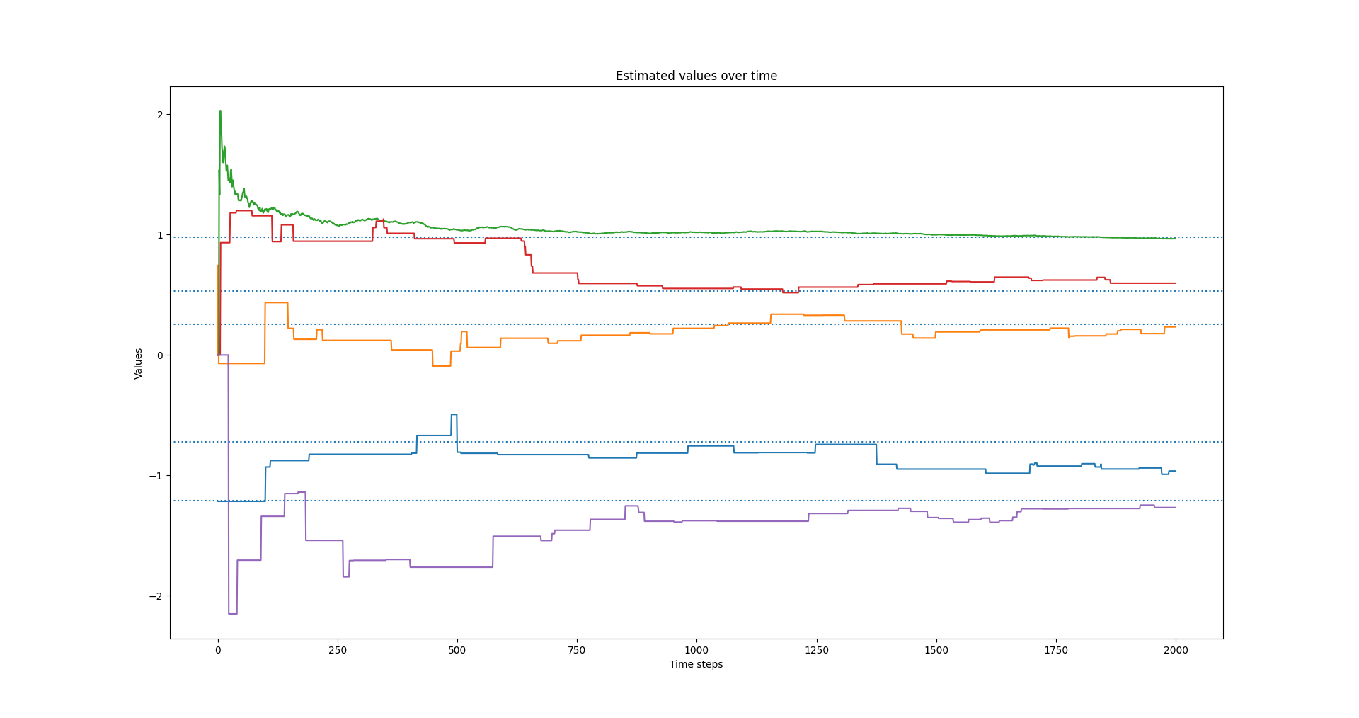
Now that we have a bandit and an agent implemented it is quite easy to run a simulation. This example simulation is a single agent with $\epsilon = 0.1$ performing 1000 updates on a single 5 arm bandit.

from agents import Agent
from bandits import Bandit


bandit = Bandit(5)
agent = Agent(bandit=bandit, epsilon=0.1, time_steps=1000)
for step in range(1000):
    agent.step()

for value in bandit.values:
    plt.axhline(value, linestyle='dotted')
plt.plot(agent.tracked_estimated_values)
plt.title("Estimated values over time")
plt.xlabel("Time steps")
plt.ylabel('Values')
plt.show()

In the figure above the true values for the arms are marked by the dashed horizontal lines. You can see that the estimated values converge on the true values as the number time steps increases (see a real RL textbook for a proof of this).

Average Performance Over Multiple Problems

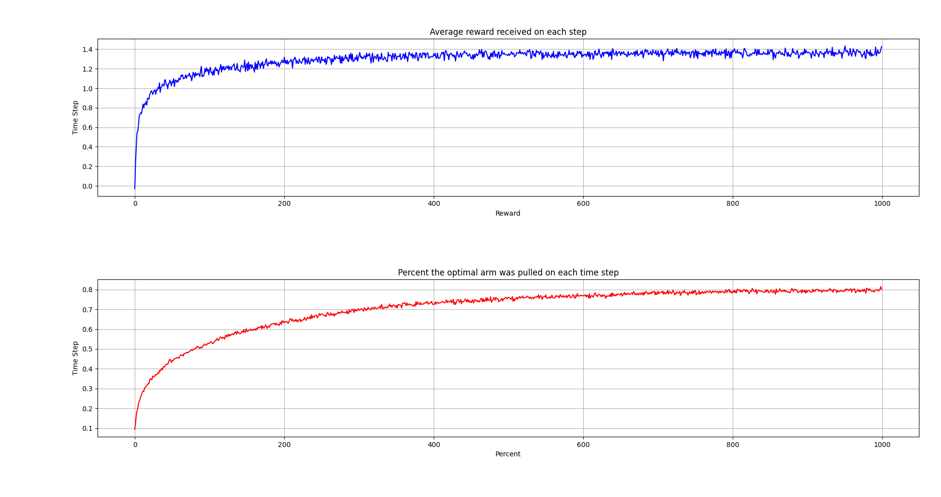
Here is the results of simulating 2000 multi armed bandit problems, each with 10 arms and $\epsilon=0.1$, and averaging the results.

import numpy as np
import matplotlib.pyplot as plt

from agents import Agent
from bandits import Bandit


# Constants
NUM_PROBLEMS = 2000     # Number of bandit problems to simulate
NUM_ARMS = 10           # Number of arms in each bandit problem
NUM_TIME_STEPS = 1000   # Number of time steps to take in each problem
EPSILON = 0.1           # Percentage of time to explore in the epsilon-greedy method

# Simulation
total_reward_each_step = np.zeros(NUM_TIME_STEPS)
optimal_pulls_each_step = np.zeros(NUM_TIME_STEPS)
for problem in range(NUM_PROBLEMS):
    bandit = Bandit(NUM_ARMS)
    agent = Agent(bandit, EPSILON, NUM_TIME_STEPS)
    for time_step in range(NUM_TIME_STEPS):
        reward, optimal = agent.step()
        total_reward_each_step[time_step] += reward
        if optimal:
            optimal_pulls_each_step[time_step] += 1

total_reward_each_step = total_reward_each_step / NUM_PROBLEMS
optimal_pulls_each_step = optimal_pulls_each_step / NUM_PROBLEMS

# Plots
plt.subplot(2, 1, 1)
plt.plot(total_reward_each_step, color='blue')
plt.title("Average reward received on each step")
plt.xlabel("Reward")
plt.ylabel("Time Step")
plt.grid()

plt.subplot(2, 1, 2)
plt.plot(optimal_pulls_each_step, color='red')
plt.title("Percent the optimal arm was pulled on each time step")
plt.xlabel("Percent")
plt.ylabel("Time Step")
plt.grid()

plt.tight_layout()
plt.show()

The first plot shows the average reward received for each pull. The second shows the percentage of time the optimal arm was pulled. Given infinite time steps, the percentage of time to optimal arm was pulled would converge to 91%.

The full code can be found on my gitlab page.